Query Performance Analysis
Query Performance Analysis
Query analysis helps users understand query execution mechanisms and identify performance bottlenecks, facilitating optimization and improving efficiency. This directly enhances user experience and resource utilization. IoTDB provides two query analysis statements: EXPLAIN and EXPLAIN ANALYZE.
EXPLAIN: Displays the query execution plan, detailing how IoTDB retrieves and processes data.EXPLAIN ANALYZE: Executes the query and provides detailed performance metrics, such as execution time and resource consumption. Unlike other diagnostic tools, it requires no deployment and focuses on single-query analysis for precise troubleshooting.
Performance Analysis Methods Comparison
| Method | Installation Difficulty | Business Impact | Functional Scope |
|---|---|---|---|
| EXPLAIN ANALYZE | Low. No additional components required; built-in SQL statement in IoTDB. | Low. Impacts only the analyzed query, with no effect on other workloads. | Supports cluster systems. Enables tracing for a single SQL query. |
| Monitoring Dashboard | Medium. Requires installation of IoTDB monitoring dashboard tool (IoTDB) and enabling monitoring services. | Medium. Metrics collection introduces additional overhead. | Supports cluster systems. Analyzes overall database query load and latency. |
| Arthas Sampling | Medium. Requires Java Arthas installation (may be restricted in internal networks; sometimes requires application restart). | High. May degrade response speed of online services due to CPU sampling. | Does n****ot supports cluster systems. Analyzes overall database query load and latency. |
1. EXPLAIN Statement
1.1 Syntax
The EXPLAIN command allows users to view the execution plan of an SQL query. It presents the plan as a series of operators, illustrating how IoTDB processes the query. The syntax is as follows, where <SELECT_STATEMENT> represents the target query:
EXPLAIN <SELECT_STATEMENT>1.2 Description
The result of EXPLAIN includes information such as data access strategies, whether filtering conditions are pushed down, and the distribution of the query plan across different nodes. This provides users with a means to visualize the internal execution logic of the query.
-- Create database
CREATE DATABASE test;

-- Create table
USE test;
CREATE TABLE t1 (device_id STRING ID, type STRING ATTRIBUTE, speed FLOAT);

-- Insert data
INSERT INTO t1(device_id, type, speed) VALUES('car_1', 'Model Y', 120.0);
INSERT INTO t1(device_id, type, speed) VALUES('car_2', 'Model 3', 100.0);

-- Execute EXPLAIN
EXPLAIN SELECT * FROM t1;
The result shows that IoTDB retrieves data from different data partitions through two TableScan nodes and aggregates the data using a Collect operator before returning it:
+-----------------------------------------------------------------------------------------------+
|                                                                               distribution plan|
+-----------------------------------------------------------------------------------------------+
|                        ┌─────────────────────────────────────────────┐                        |
|                        │OutputNode-4                                 │                        |
|                        │OutputColumns-[time, device_id, type, speed] │                        |
|                        │OutputSymbols: [time, device_id, type, speed]│                        |
|                        └─────────────────────────────────────────────┘                        |
|                                               │                                               |
|                                               │                                               |
|                        ┌─────────────────────────────────────────────┐                        |
|                        │Collect-21                                   │                        |
|                        │OutputSymbols: [time, device_id, type, speed]│                        |
|                        └─────────────────────────────────────────────┘                        |
|                       ┌───────────────────────┴───────────────────────┐                       |
|                       │                                               │                       |
|┌─────────────────────────────────────────────┐                  ┌───────────┐                 |
|│TableScan-19                                 │                  │Exchange-28│                 |
|│QualifiedTableName: test.t1                  │                  └───────────┘                 |
|│OutputSymbols: [time, device_id, type, speed]│                        │                       |
|│DeviceNumber: 1                              │                        │                       |
|│ScanOrder: ASC                               │ ┌─────────────────────────────────────────────┐|
|│PushDownOffset: 0                            │ │TableScan-20                                 │|
|│PushDownLimit: 0                             │ │QualifiedTableName: test.t1                  │|
|│PushDownLimitToEachDevice: false             │ │OutputSymbols: [time, device_id, type, speed]│|
|│RegionId: 2                                  │ │DeviceNumber: 1                              │|
|└─────────────────────────────────────────────┘ │ScanOrder: ASC                               │|
|                                                │PushDownOffset: 0                            │|
|                                                │PushDownLimit: 0                             │|
|                                                │PushDownLimitToEachDevice: false             │|
|                                                │RegionId: 1                                  │|
|                                                └─────────────────────────────────────────────┘|
+-----------------------------------------------------------------------------------------------+
2. EXPLAIN ANALYZE Statement
2.1 Syntax
The EXPLAIN ANALYZE statement provides detailed performance metrics by executing the query and analyzing its runtime behavior. The syntax is as follows:
EXPLAIN ANALYZE [VERBOSE] <SELECT_STATEMENT>SELECT_STATEMENTcorresponds to the query statement to be analyzed.VERBOSE(optional): Prints detailed analysis results. Without this option, some metrics are omitted.
2.2 Description
Explain Analyze is a performance analysis SQL built into the IoTDB query engine. Unlike Explain, it runs the query and collects execution metrics, enabling users to trace performance bottlenecks, observe resource usage, and conduct precise performance tuning.
The output includes detailed statistics such as query planning time, execution time, data partitioning, and resource consumption:
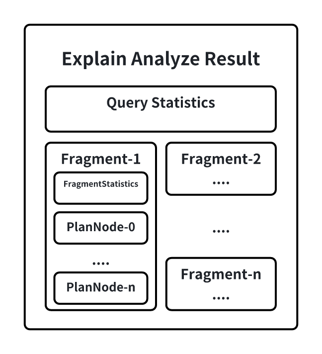
2.3 Detailed Breakdown of EXPLAIN ANALYZE Results
QueryStatistics
QueryStatistics contains high-level statistics about the query execution, including the time spent in each planning stage and the number of query shards.
- Analyze Cost: Time spent in the SQL analysis phase, including
FetchPartitionCostandFetchSchemaCost. - Fetch Partition Cost: Time spent fetching partition tables.
- Fetch Schema Cost: Time spent fetching schema and performing permission checks.
- Logical Plan Cost: Time spent building the logical plan.
- Logical Optimization Cost: Time spent optimizing the logical plan.
- Distribution Plan Cost: Time spent building the distributed execution plan.
- Fragment Instance Count: The total number of query shards. Each shard's information is output individually.
FragmentInstance
A FragmentInstance is a wrapper for a query shard in IoTDB. Each query shard outputs its execution information in the result set, including FragmentStatistics and operator information. FragmentStatistics provides detailed metrics about the shard's execution, including:
- Total Wall Time: The physical time from the start to the end of the shard's execution.
- Cost of initDataQuerySource: Time spent building the query file list.
- Seq File (unclosed): Number of unclosed (memtable) sequential files.
- Seq File (closed): Number of closed sequential files.
- UnSeq File (unclosed): Number of unclosed (memtable) unsequential files.
- UnSeq File (closed): Number of closed unsequential files.
- Ready Queued Time: Total time the shard's tasks spent in the ready queue (tasks are not blocked but lack query execution thread resources).
- Blocked Queued Time: Total time the shard's tasks spent in the blocked queue (tasks are blocked due to resources like memory or upstream data not being sent).
Since V2.0.9, the following information will be added to FragmentInstance:
OutputPlanNodeId: Indicates the downstream node that receives data corresponding to the sink node. Only present in sink nodes.sizeInBytes: Represents the size in bytes of TsBlocks received in exchange nodes (only data size is counted). Only present in exchange nodes.- Data filtering‑related fields for
tableScannodes. Valid only when filter pushdown is applied to tableScan, and only present in tableScan nodes:TimeSeriesIndexFilteredRows: Number of rows filtered out by TimeseriesMetadataChunkIndexFilteredRows: Number of rows filtered out by ChunkMetadataPageIndexFilteredRows: Number of rows filtered out by PageHeader internal filteringRowScanFilteredRows: Number of rows filtered out during per-row data inspection. Only displayed whenverboseis enabled.
BloomFilter-Related Metrics
Bloom filters help determine if a sequence exists in a TsFile. They are stored at the end of each TsFile.
- loadBloomFilterFromCacheCount: Number of times the BloomFilterCache was hit.
- loadBloomFilterFromDiskCount: Number of times BloomFilter was read from disk.
- loadBloomFilterActualIOSize: Disk I/O used when reading BloomFilter (in bytes).
- loadBloomFilterTime: Total time spent reading BloomFilter and checking if a sequence exists (in milliseconds).
TimeSeriesMetadata-Related Metrics
TimeSeriesMetadata contains indexing information for sequences in a TsFile. Each TsFile has one metadata entry per sequence.
- loadTimeSeriesMetadataDiskSeqCount: Number of TimeSeriesMetadata entries loaded from closed sequential files.
- Usually equals the number of closed sequential files but may be lower if operators like
LIMITare applied.
- Usually equals the number of closed sequential files but may be lower if operators like
- loadTimeSeriesMetadataDiskUnSeqCount: Number of TimeSeriesMetadata entries loaded from closed unsequential files.
- loadTimeSeriesMetadataDiskSeqTime: Time spent loading sequential TimeSeriesMetadata from disk.
- Not all loads involve disk I/O, as cache hits may reduce access time.
- loadTimeSeriesMetadataDiskUnSeqTime: Time spent loading unsequential TimeSeriesMetadata from disk.
- loadTimeSeriesMetadataFromCacheCount: Number of cache hits when accessing TimeSeriesMetadata.
- loadTimeSeriesMetadataFromDiskCount: Number of times TimeSeriesMetadata was read from disk.
- loadTimeSeriesMetadataActualIOSize: Disk I/O used for TimeSeriesMetadata reads (in bytes).
Mods File-Related Metrics
- TimeSeriesMetadataModificationTime: Time spent reading modification (mods) files.
Chunk-Related Metrics
Chunks are the fundamental units of data storage in TsFiles.
- constructAlignedChunkReadersDiskCount: Number of Chunks read from closed TsFiles.
- constructAlignedChunkReadersDiskTime: Total time spent reading Chunks from closed TsFiles (including disk IO and decompression).
- pageReadersDecodeAlignedDiskCount: Number of pages decoded from closed TsFiles.
- pageReadersDecodeAlignedDiskTime: Total time spent decoding pages from closed TsFiles.
- loadChunkFromCacheCount: Number of times ChunkCache was hit.
- For aligned devices, each component (including the time column) requests the cache separately. Therefore,
(loadChunkFromCacheCount + loadChunkFromDiskCount)equalstsfile number * subSensor number (including the time column) * avg chunk number in each TsFile.
- For aligned devices, each component (including the time column) requests the cache separately. Therefore,
- loadChunkFromDiskCount: Number of times Chunks were read from disk.
- loadChunkActualIOSize: Disk I/O used when reading Chunks (in bytes).
2.4 Special Notes
Query Timeout Scenario with EXPLAIN ANALYZE
Since EXPLAIN ANALYZE runs as a special query type, it cannot return results if execution times out. To aid troubleshooting, IoTDB automatically enables a timed logging mechanism that periodically records partial results to a dedicated log file (logs/log_explain_analyze.log). This mechanism requires no user configuration.
- The logging interval is dynamically calculated based on the query's timeout duration, ensuring at least two log entries before the timeout occurs.
- Users can examine the log file to identify potential causes of the timeout.
2.5 Example
The following example demonstrates how to use EXPLAIN ANALYZE:
-- Create Database
CREATE DATABASE test;

-- Create Table
USE test;
CREATE TABLE t1 (device_id STRING ID, type STRING ATTRIBUTE, speed FLOAT);

-- Insert Data
INSERT INTO t1(device_id, type, speed) VALUES('car_1', 'Model Y', 120.0);
INSERT INTO t1(device_id, type, speed) VALUES('car_2', 'Model 3', 100.0);

-- Execute EXPLAIN ANALYZE
EXPLAIN ANALYZE VERBOSE SELECT * FROM t1;
Output (Simplified):
+-----------------------------------------------------------------------------------------------+
| Explain Analyze|
+-----------------------------------------------------------------------------------------------+
|Analyze Cost: 38.860 ms |
|Fetch Partition Cost: 9.888 ms |
|Fetch Schema Cost: 54.046 ms |
|Logical Plan Cost: 10.102 ms |
|Logical Optimization Cost: 17.396 ms |
|Distribution Plan Cost: 2.508 ms |
|Dispatch Cost: 22.126 ms |
|Fragment Instances Count: 2 |
| |
|FRAGMENT-INSTANCE[Id: 20241127_090849_00009_1.2.0][IP: 0.0.0.0][DataRegion: 2][State: FINISHED]|
| Total Wall Time: 18 ms |
| Cost of initDataQuerySource: 6.153 ms |
| Seq File(unclosed): 1, Seq File(closed): 0 |
| UnSeq File(unclosed): 0, UnSeq File(closed): 0 |
| ready queued time: 0.164 ms, blocked queued time: 0.342 ms |
| Query Statistics: |
| loadBloomFilterFromCacheCount: 0 |
| loadBloomFilterFromDiskCount: 0 |
| loadBloomFilterActualIOSize: 0 |
| loadBloomFilterTime: 0.000 |
| loadTimeSeriesMetadataAlignedMemSeqCount: 1 |
| loadTimeSeriesMetadataAlignedMemSeqTime: 0.246 |
| loadTimeSeriesMetadataFromCacheCount: 0 |
| loadTimeSeriesMetadataFromDiskCount: 0 |
| loadTimeSeriesMetadataActualIOSize: 0 |
| constructAlignedChunkReadersMemCount: 1 |
| constructAlignedChunkReadersMemTime: 0.294 |
| loadChunkFromCacheCount: 0 |
| loadChunkFromDiskCount: 0 |
| loadChunkActualIOSize: 0 |
| pageReadersDecodeAlignedMemCount: 1 |
| pageReadersDecodeAlignedMemTime: 0.047 |
| [PlanNodeId 43]: IdentitySinkNode(IdentitySinkOperator) |
| CPU Time: 5.523 ms |
| output: 2 rows |
| HasNext() Called Count: 6 |
| Next() Called Count: 5 |
| Estimated Memory Size: : 327680 |
| [PlanNodeId 31]: CollectNode(CollectOperator) |
| CPU Time: 5.512 ms |
| output: 2 rows |
| HasNext() Called Count: 6 |
| Next() Called Count: 5 |
| Estimated Memory Size: : 327680 |
| [PlanNodeId 29]: TableScanNode(TableScanOperator) |
| CPU Time: 5.439 ms |
| output: 1 rows |
| HasNext() Called Count: 3
| Next() Called Count: 2 |
| Estimated Memory Size: : 327680 |
| DeviceNumber: 1 |
| CurrentDeviceIndex: 0 |
| [PlanNodeId 40]: ExchangeNode(ExchangeOperator) |
| CPU Time: 0.053 ms |
| output: 1 rows |
| HasNext() Called Count: 2 |
| Next() Called Count: 1 |
| Estimated Memory Size: : 131072 |
| |
|FRAGMENT-INSTANCE[Id: 20241127_090849_00009_1.3.0][IP: 0.0.0.0][DataRegion: 1][State: FINISHED]|
| Total Wall Time: 13 ms |
| Cost of initDataQuerySource: 5.725 ms |
| Seq File(unclosed): 1, Seq File(closed): 0 |
| UnSeq File(unclosed): 0, UnSeq File(closed): 0 |
| ready queued time: 0.118 ms, blocked queued time: 5.844 ms |
| Query Statistics: |
| loadBloomFilterFromCacheCount: 0 |
| loadBloomFilterFromDiskCount: 0 |
| loadBloomFilterActualIOSize: 0 |
| loadBloomFilterTime: 0.000 |
| loadTimeSeriesMetadataAlignedMemSeqCount: 1 |
| loadTimeSeriesMetadataAlignedMemSeqTime: 0.004 |
| loadTimeSeriesMetadataFromCacheCount: 0 |
| loadTimeSeriesMetadataFromDiskCount: 0 |
| loadTimeSeriesMetadataActualIOSize: 0 |
| constructAlignedChunkReadersMemCount: 1 |
| constructAlignedChunkReadersMemTime: 0.001 |
| loadChunkFromCacheCount: 0 |
| loadChunkFromDiskCount: 0 |
| loadChunkActualIOSize: 0 |
| pageReadersDecodeAlignedMemCount: 1 |
| pageReadersDecodeAlignedMemTime: 0.007 |
| [PlanNodeId 42]: IdentitySinkNode(IdentitySinkOperator) |
| CPU Time: 0.270 ms |
| output: 1 rows |
| HasNext() Called Count: 3 |
| Next() Called Count: 2 |
| Estimated Memory Size: : 327680 |
| [PlanNodeId 30]: TableScanNode(TableScanOperator) |
| CPU Time: 0.250 ms |
| output: 1 rows |
| HasNext() Called Count: 3 |
| Next() Called Count: 2 |
| Estimated Memory Size: : 327680 |
| DeviceNumber: 1 |
| CurrentDeviceIndex: 0 |
+-----------------------------------------------------------------------------------------------+2.6 FAQs
Differences Between WALL TIME and CPU TIME
- CPU TIME (also known as processor time or CPU utilization time) refers to the actual time a program spends executing on the CPU, reflecting the amount of CPU resources consumed.
- WALL TIME (also known as elapsed time or physical time) refers to the total time from the start to the end of a program's execution, including all waiting periods.
Key Scenarios:
- WALL TIME < CPU TIME: This occurs when multiple threads are used for parallel execution. For example, if a query shard runs for 10 seconds in real-world time using two threads, the CPU time would be 20 seconds (10 seconds × 2 threads), while the wall time would remain 10 seconds.
- WALL TIME > CPU TIME: This typically happens due to resource contention or insufficient query threads:
- Blocked by Resource Constraints: If a query shard is blocked (e.g., due to insufficient memory for data transfer or waiting for upstream data), it remains in the Blocked Queue, accumulating wall time without consuming CPU time.
- Insufficient Query Threads: If 20 query shards are running concurrently but only 16 query threads are available, 4 shards will be placed in the Ready Queue, waiting for execution. During this waiting period, wall time continues to elapse, but no CPU time is consumed.
Additional Considerations for EXPLAIN ANALYZE
EXPLAIN ANALYZE introduces minimal overhead, as it runs in a separate thread to collect query statistics. These metrics are generated by the system regardless of whether EXPLAIN ANALYZE is executed; the command simply retrieves them for user inspection.
Additionally, EXPLAIN ANALYZE iterates through the result set without producing output. Therefore, the reported execution time closely reflects the actual query execution time, with negligible deviation.
Key Metrics for I/O Time
The following metrics are crucial for evaluating I/O performance during query execution:
loadBloomFilterActualIOSizeloadBloomFilterTimeloadTimeSeriesMetadataAlignedDisk[Seq/Unseq]TimeloadTimeSeriesMetadataActualIOSizealignedTimeSeriesMetadataModificationTimeconstructAlignedChunkReadersDiskTimeloadChunkActualIOSize
These metrics were detailed in previous sections. While TimeSeriesMetadata loading is tracked separately for sequential and unsequential files, chunk reading is not currently differentiated. However, the proportion of sequential versus unsequential data can be inferred from TimeSeriesMetadata statistics.
Impact of Unsequential Data on Query Performance
Unsequential data can negatively affect query performance in the following ways:
- Additional Merge Sort in Memory: Unsequential data requires an additional merge sort in memory, which is generally a short operation since it involves pure CPU operations.
- Overlap in Time Ranges: Unsequential data can cause time-range overlaps between data chunks, rendering statistical information unusable:
- Inability to Skip Chunks: If a query involves value filtering conditions, statistical information cannot be used to skip entire chunks that do not meet the criteria. However, this is less impactful if the query only involves time filtering.
- Inability to Compute Aggregates Directly: Statistical information cannot be used to directly compute aggregate values without reading the data.
Currently, there is no direct method to measure the performance impact of unsequential data. The only approach is to compare query performance before and after merging the unsequential data. However, even after merging, the query still incurs I/O, compression, and decoding overhead, meaning the execution time will not decrease significantly.
Why EXPLAIN ANALYZE Results Are Not Logged on Query Timeout
If EXPLAIN ANALYZE results are missing from the log_explain_analyze.log file after a query timeout, the issue may stem from an incomplete system upgrade. Specifically, if the lib package was updated without updating the conf/logback-datanode.xml file, the logging configuration may be outdated.
Solution:
- Replace the
conf/logback-datanode.xmlfile with the updated version. - A system restart is not required, as the new configuration will be hot-loaded automatically.
- Wait approximately one minute, then re-execute the
EXPLAIN ANALYZEstatement with theVERBOSEoption to confirm proper logging.